Coding Theory: Hamming Distance, Code, and Bound

Attempting to dive into the basics of coding theory

Some time ago I wrote an article trying to dive into how QR codes actually work by trying to decode a simple one. All went well until I got to the part of understanding how the error correction bits work and how they help restore any lost information. While the pseudocode is available online and it would be doable to write your own text to QR encoder (that’s what she said), I couldn’t grasp the maths behind the Reed-Solomon codes and how it helps with error correction. It seems I was missing a lot of concepts and theory.

So here I am, starting a new series of articles diving into Coding Theory. From Hamming distance, parity checks, linear codes, Reed-Solomon codes to BCH and maybe beyond? We’ll see how long my curiosity lasts.

This article will talk about:

• what is noise, error detection and error correction

• definitions - hamming distance, ball, volume, code dimension, rate, weight and hamming bound

And at the end of it, you should be able to:

• find and use the Hamming distance for a code

• understand the trade-off between rate and distance

The Goal of Coding Theory

One of the main goals of coding theory is developing methods to detect/correct errors caused by the transmission of information through noisy channels.

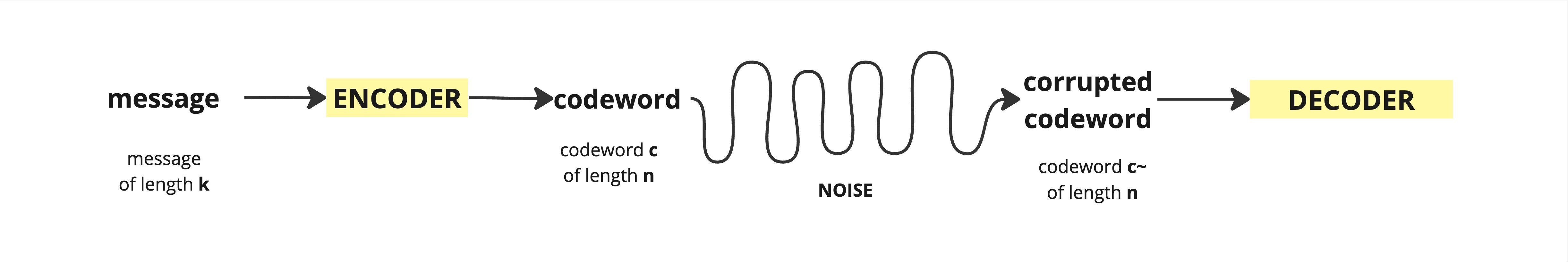
message m of length k → (encoding) codeword c  → (channel) received word c’ →  (decoding) message m’ of length n

Let’s say we have a message m of length k which we are going to encode (somehow) and get a word c of length n. Here n > k as we are adding redundancy data to our original message. We transmit the encoded word c through some communication channel but some of the bits get corrupted and so we receive a corrupted codeword c~ of length n.

We are concerned about 4 things:

1. Handling the communication noise.

2. Recovering the initial message.

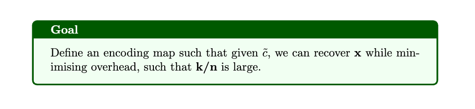
3. Minimising overhead, meaning k/n should be large.

4. Being able to do the above through an encoding method that is efficient.

Binary bit-error correcting codes

To start off, there are a couple of assumptions we’ll make. All messages that we want to send are binary strings and we will only be transmitting binary strings across the channel and the only errors that occur are bit-errors, which consist of replacing 0 by 1 or 1 by 0.

Let’s start by providing the formal definition of what a codeword c is.

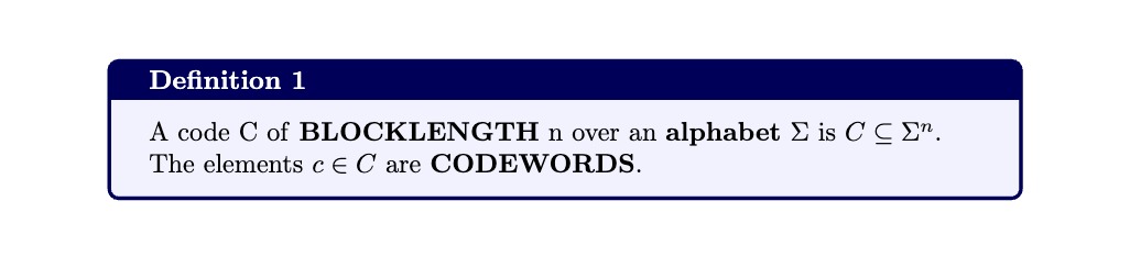
Example 1 An example would be the following where C is a matrix of vectors of length 4 over an alphabet {0,1}. C is a code which has 8 codewords, each of length 4 and all digits are either 0 or 1. Such codes are called binary codes.

Example 2

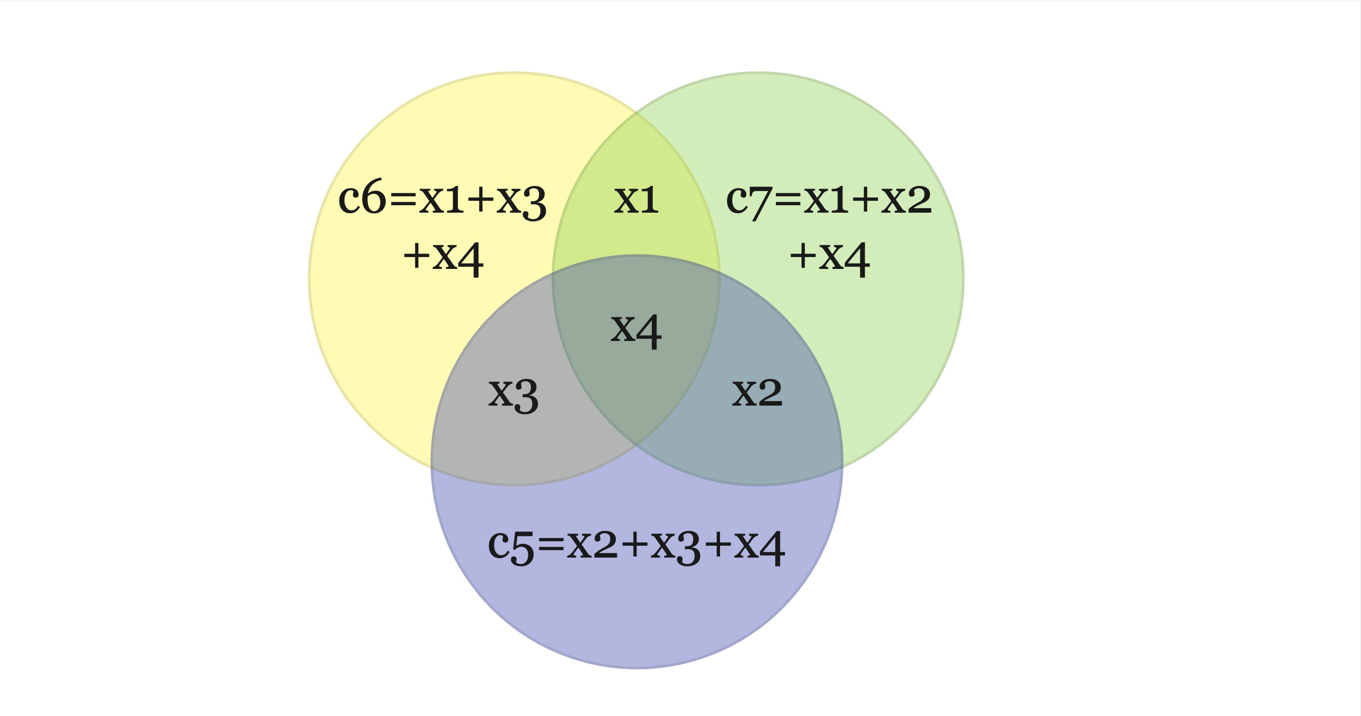
Suppose we have the following code (also known as the Hamming Code)

Then C is a binary code of blocklength 7. There is a nice way to visualise the bove encoding using 3 circles. Our message bits will be at the intersection of any 2 circles and all the other 3 parity bits ((x2,x3,x4)%2, etc) correspond to the remaining empty cells. You can also notice that each circle sums up to 0mod2.

The Hamming Code is capable of detecting up to two simultaneous bit errors and correcting single-bit errors. Let’s say we get the following corrupted code word c~={0111010}. Are we able to figure out c? One way to check which bit got flipped is to use the same circle representation above and use the bits that we got:

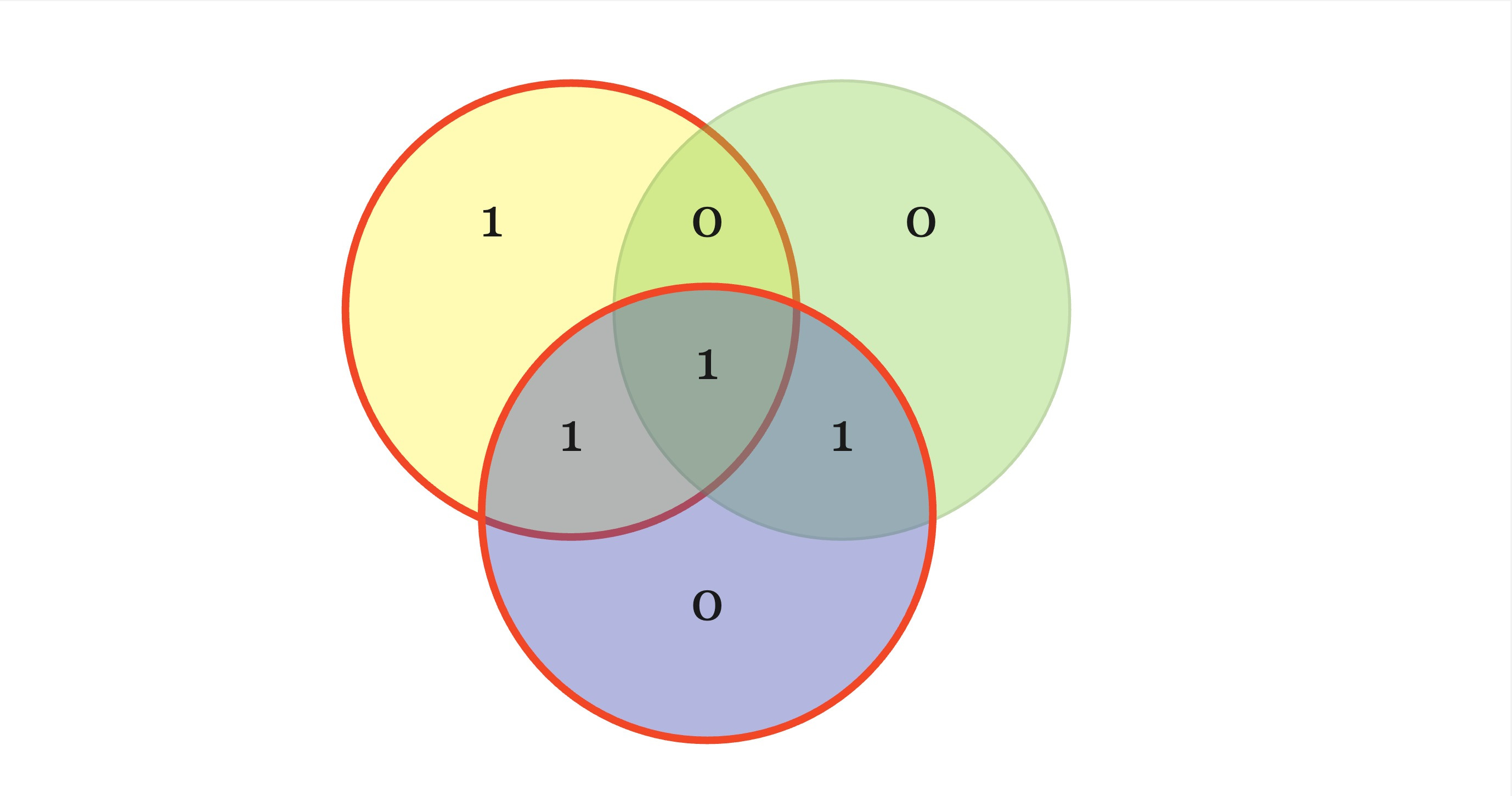
We know that the sum of the bits in each circle should sum up to 0mod%2 but the yellow and blue one don’t, which means the bit at their intersection (aka the 3rd bit) has been corrupted. So now we know the corrected codeword is c={0101010}

Let’s continue with some more formal definitions. The Hamming Distance between two strings is the number of positions in which they differ.

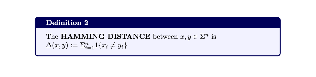
For example Δ(001, 100) = 2.

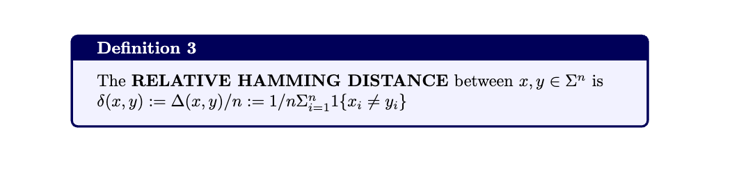
The Relative Hamming Distance and the Minimum Distance are defined as:

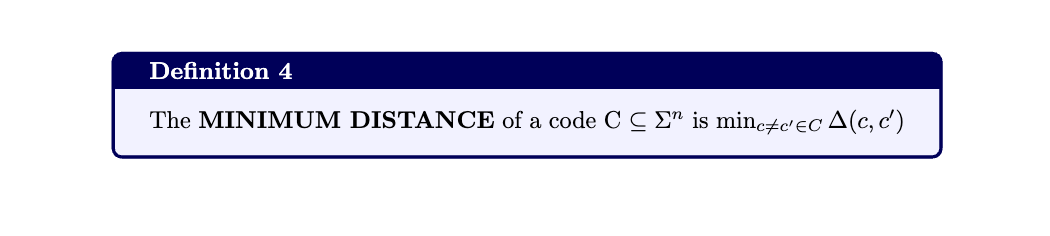
The distance of a code is the minimum Hamming distance between two distinct codewords in the code.

For example, the distance of {001, 010, 100, 111} is 2.

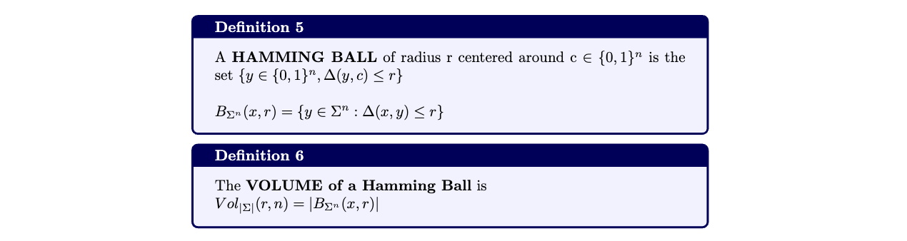
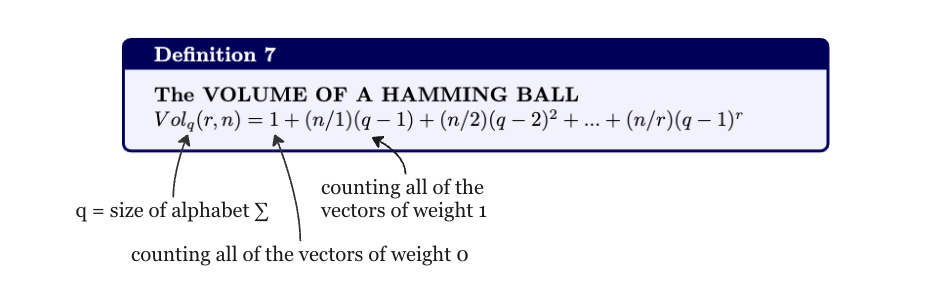
Another definition of the volume of a Hamming Ball can be defined as:

Example Given the following code C = {001,101,100,111} where first 2 bits are information bits, the Hamming Ball can be calculated as follows:

• Calculate the Hamming Distance: For each codeword, calculate the Hamming distance to all other codewords within the specified radius. Let's say we want to calculate the Hamming ball of radius 1.

  • For codeword 001: Hamming distance of 1 to 010 and 100.

  • For codeword 010: Hamming distance of 1 to 001 and 111.

  • For codeword 100: Hamming distance of 1 to 001 and 111.

  • For codeword 111: Hamming distance of 1 to 010 and 100.

• Count the Codewords within the Radius: Count the number of codewords that fall within the specified radius from each codeword.

  • For codeword 001: 2 codewords (010, 100) within radius 1.

  • For codeword 010: 2 codewords (001, 111) within radius 1.

  • For codeword 100: 2 codewords (001, 111) within radius 1.

  • For codeword 111: 2 codewords (010, 100) within radius 1.

• Calculate the Volume: The volume of the Hamming ball is the sum of the counts of codewords within the radius from each codeword.

  • Volume = 2 (from 001) + 2 (from 010) + 2 (from 100) + 2 (from 111) = 8.

Detecting and Correcting Errors

The error-correcting capability of a code refers to its ability to detect and correct errors that occur during transmission. A code with a larger minimum distance can correct more errors.

Detecting errors involves finding out if an error has occurred.

We say a code can detect d errors if the following holds:
Whenever a codeword is transmitted across a channel capable of producing d bit-errors, it is possible to deduce whether an error occurred using only the received word.

If the distance of a code is d, then the code can detect exactly d−1 errors.

Proof If a channel can produce at most d−1 bit-errors, it cannot turn one codeword into another by flipping bits, because the minimum Hamming distance between any two codewords is at least d. Thus, if the received word c’ is not in the code, we can deduce that some errors occurred. The code is not guaranteed to detect d errors, because one codeword can be transformed into another by d bit-errors.

We say a code can correct d errors if the following holds:
Whenever a codeword is transmitted across a channel capable of producing d bit-errors, one can deduce which codeword was sent using only the received word.

If the distance of a code is d, then the code can correct exactly ⌊(d − 1)/2⌋ errors.

Proof Suppose C is a code of distance d, and a codeword c is sent across a channel capable of producing at most ⌊(d − 1)/2⌋ bit-errors. Consider we have received the word c’ that is the result of transmitting the codeword c and introducing some errors. We claim that c is the only codeword within distance ⌊(d − 1)/2⌋ of c’. If there were another codeword, say c’’, then it would mean Δ(c,c’’) ≤ 2⌊(d − 1)/2⌋ ≤ d-1 (which is a contradiction based on the properties of non-overlapping neighborhoods)

Example The following code C = {001,101,100,111} has distance 2 which means it can detect 1 error, but it can correct 0 errors.

A code with minimum Hamming distance d between its codewords, can:

• detect at most d-1 errors

• correct at most ⌊(d − 1)/2⌋ errors

How much information can we send: the Rate

The rate of a code is defined as the ratio of the number of information bits to the total number of bits in a codeword, which is a value between [0,1]. The closer to 1 the better.

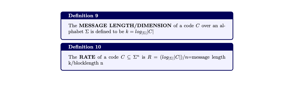
Given the following code C={000,101,011,110} where let’s say we use an encoding where the 2 bits are the information bits. This means our rate is:
R = number of information bits/length of the codeword = 2/3

In coding theory, higher-rate codes are desirable because they allow more information to be transmitted per unit of time or bandwidth. However, increasing the rate often comes at the cost of reduced error-correction capability, as higher-rate codes typically have shorter minimum distances. Therefore, there is often a trade-off between rate and error-correction performance in code design.

Rate and Distance Trade-off: the Hamming Bound

How does rate and distance influence each other?

• Higher Rate, Lower Distance: Increasing the rate of a code often comes at the expense of reducing its distance. This is because increasing the rate typically involves reducing redundancy in the codewords, which means fewer bits are available for error detection and correction. As a result, the distance of the code decreases, making it less capable of correcting errors.

• Lower Rate, Higher Distance: Conversely, decreasing the rate of a code allows for more redundancy to be added to the codewords, which increases the distance of the code. This provides better error-correcting capability but at the cost of transmitting fewer information bits per codeword.

Increasing the rate improves efficiency but may reduce error-correcting capability, while increasing the distance enhances error-correcting capability but may reduce efficiency.

So what is the best trade-off between rate and distance? The Hamming Bound establishes some limitations of how good this trade off can be.

Let’s try and visualise this. Let’s say we have our alphabet ∑ with codewords c in code C, where C has distance d. All of the codewords neighborhoods are non-overlapping since each ball has radius ⌊(d − 1)/2⌋ and the distance between any 2 codewords is d.

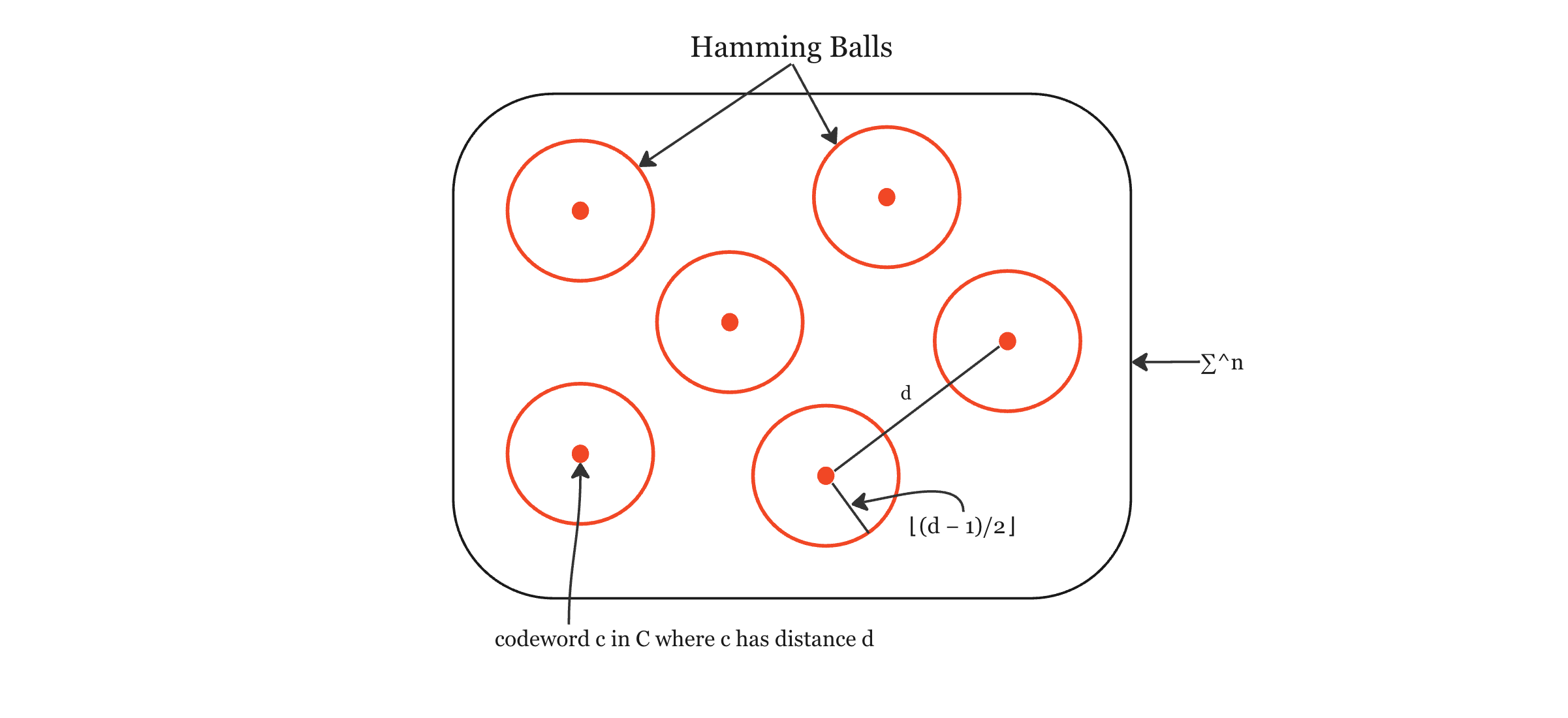
From this we can get an idea of what the Hamming Bound is all about. We have those |C| disjoint balls of radius ⌊(d − 1)/2⌋but all of those balls need to fit in ∑^n, so we can’t have too many balls. Therefore, we can’t have too many codewords and the rate of the code can’t be too big. All those disjoint Hamming Balls need to live in ∑^n

Using the definition for the volume of the Hamming Ball, we can define the following:

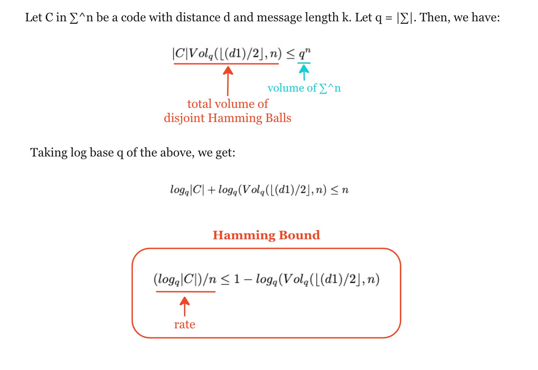
The Hamming Bound gives us a bound in terms of the distance and rate and is important in coding theory as it places an upper limit on the number of distinct codewords that can be encoded using a block of symbols of particular length, to provide a specified error-correcting capability.

Conclusion

As this article is getting quite long and there are still a lot of things to talk about we’ll stop here. Now that we have most of the definitions and theorems defined, next article will cover more practical examples on how to calculate the Hamming Bound for different codes. We’ll also discuss what are generator and parity matrixes and how to decode corrupted codewords.

Resources:

• Huge appreciation to Mary Wootters’ for her free Algebraic Coding Theory YT Lessons